Magnon spectra and noncollinear magnetism
Tutorial 0: Spin wave stiffness
The spin wave stiffness and the related property exchange stiffness provides the bridge between atomistic spin dynamics and micromagnetism.
A setup for bcc Fe where the stiffness can be calculated can be seen below
simid bccFe100
ncell     36       36      36                 System size
BC        P         P         P                 Boundary conditions (0=vacuum, P=periodic)
cell         -0.5000000000    0.5000000000    0.5000000000
              0.5000000000   -0.5000000000    0.5000000000
              0.5000000000    0.5000000000   -0.5000000000
Sym       1                                     Symmetry of lattice (0 for no, 1 for cubic, 2 for 2d cubic, 3 for hexagonal)

posfile   ./posfile
posfiletype D
momfile   ./momfile
exchange  ./jASD2S

Initmag   3                                     Initial config of moments (1=random, 2=cone, 3=spec., 4=file)

do_avrg   Y                                     Measure averages
do_cumu Y
plotenergy 1

do_ams Y
do_magdos Y
qpoints D
qfile ./qfile.kpath

do_stiffness Y
eta_max 12
eta_min 6
alat 2.87e-10
Notice that we actually have no ip_mode nor mode sections, because here we are actually not interested in running any simulation.
The posfile and momfile are here as follows
1 1 0.000000 0.000000 0.000000
1 1 2.2459 0.0 0.0 1.0 0.0
The exchange interaction file jASD2S can be downloaded from here .
Calculate the spin wave stiffness for the system and examine how the results depend on the choice of
eta_maxandeta_min.
The output from the stiffness calculations are found in the asd_micro.bccFe100.out file.
Tutorial 0b: Spin wave scripts
Even though the calculation of magnon spectra will be practiced on in more detail enough,
one can also use the setup above to quickly showcase the functionality of the preQ.py and postQ.py scripts.
These scripts are available in the repository but are continiously evolving. Up-to-date scripts are provided here: preQ.py and postQ.py
Use the
preQ.pyscript to setup a k-space path for the spin wave dispersion in bcc Fe, run the system, and plot the resultingams.pngby usingpostQ.py.
- Optional:
The
preQ.pyscript provides several k-space paths. Compare the calculated magnon DOSmagdos.bccFe100.outwhen using eitherqpoints Dandqfile ./qfile.kpathorqpoints Randqfile ./qfile.reduced.
Tutorial 1: Fe in bcc and fcc crystal structures
Collinear magnon spectra and influence of uniaxial anisotropy
This example shows how to calculate the spin wave spectrum of the standard examples Fe bcc and Fe fcc and to understand the influence of the number of atoms per unit cell on the spectra together with the influence of the uniaxial anisotropy. Files are found in Fe folder.
Crystal & magnetic structure
Using the lines below with the indicated files, the crystal and magnetic structure are readily available, so that an Fe bcc system is created.
simid bccFe100
ncell     10        10       10                 System size
BC        P         P         P                 Boundary conditions (0=vacuum, P=periodic)
cell      1.00000   0.00000   0.00000
          0.00000   1.00000   0.00000
          0.00000   0.00000   1.00000
Sym       0      Symmetry of lattice (0 for no, 1 for cubic, 2 for 2d cubic, 3 for hexagonal)
posfile    ./posfile
momfile    ./momfile
exchange   ./jfile
anisotropy ./kfile
do_prnstruct 2          Flag to print lattice structure (0=off/1=on/2=print only coordinates)
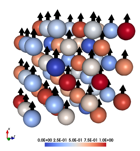
Fig 1. Lattice and magnetic texture.
Thermalizing the system
Using the lines below, the systems is driven to the ground state.
ip_mode   M
ip_mcanneal 1
10000 0.001 1.00e-16 0.95

mode      M
Temp      0.001          K                      Temperature of the system
hfield    0.00000   0.00000   0.00000           Static H field
mcNstep   50000                                 MC steps
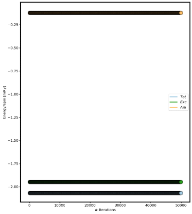
Fig 2. Energy versus number of iterations.
Spin wave spectrum
We calculate the spin wave spectrum (in this case, a collinear adiabatic magnon spectra (AMS)) at the list of Q points qfile. Use qmaker script.
do_ams Y                         Collinear Adiabatic magnon spectra
qpoints D                        Direct coordinates
qfile ./qfile                    Path along the high symmetry points in the reciprocal space
The first Brilluoin zone of a body centered cubic lattice
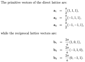
Fig 3. Primitive and reciprocal lattice vectors in bcc.
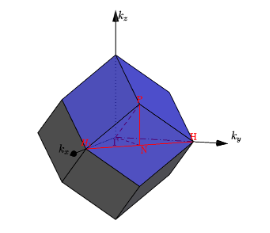
Fig 4. BCC 1st Brilluoin zone.
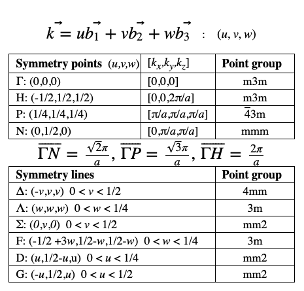
Fig 5. High symmetry points.
Plotting the spectrum
Use the UppASD graphical interface (ASDGUI) or the script enclosed in this course (plotsqw_course). Use option 2.
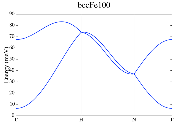
Fig 6. Adiabatic magnon spectra.
Questions and exercises:
Does the spectra follow the analytical expression?
Why the spectra is shift it up?
Plot the spectra without the gap around the center zone.
Why there are two branches, 1 acoustic and 1 optical?
Plot the spectrum for Fe fcc. Why now there is just 1 branch? Is it following the analytical expression?
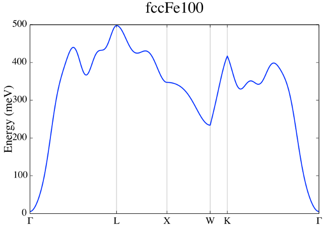
Fig 7. Adiabatic magnon spectra of Fe FCC.
Tutorial 2: FM Heisenberg nearest-neighbour spin chain
Collinear adiabatic magnon spectra and S(q,w)
The following tutorial shows every step necessary to calculate spin wave spectrum and S(q,w) through the simple example of the ferromagnetic spin chain. Notice that the classical magnetic ground state of the Hamiltonian defined in this example is where every spin have the same direction, the direction is arbitrary since the Hamiltonian is isotropic. Files are found in HeisChain folder.
Crystal & magnetic structure
Using the lines below with the indicated files, the crystal and magnetic structure are readily available, so that an 1D Heisenberg chain is created.
simid     HeisWire                              System name
ncell     1         1         100               System size (in terms of unit cells)
BC        0         0         P                 Boundary conditions (0=vacuum,P=periodic)
cell      1.00000   0.00000   0.00000
         0.00000   1.00000   0.00000
         0.00000   0.00000   1.00000
Sym       1                                     Symmetry of lattice (0 for no, 1 for cubic, 2 for 2d cubic, 3 for hexagonal)

posfile   ./posfile                             Position file
exchange  ./jfile                               Exchange file
momfile   ./momfile                             Moment file
do_prnstruct 1          Flag to print lattice structure (0=off/1=on/2=print only coordinates)
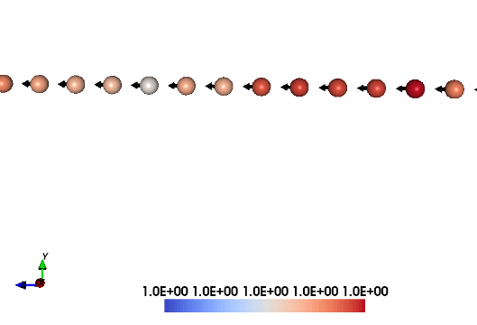
Fig 1. Crystal and magnetic texture.
Spin dynamics
Using the lines below, the systems is driven to the ground state by spin dynamics.
Mensemble 1                                     Number of samples in ensemble averaging
Initmag   3                                     (1=random, 2=cone, 3=spec., 4=file)

ip_mode   S                                     Initial phase parameters
ip_nphase 1
20000 1.0e-3 1e-16 4.0

mode      S                                     S=SD, M=MC
temp      1.0e-3                                Measurement phase parameters
damping   0.0010                                --
Nstep     40000                                 --
timestep  1.000e-15                             --
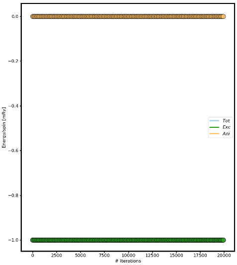
Fig 2. Energy versus number of iterations.
Spin wave spectrum
We calculate the spin wave spectrum (in this case, a collinear adiabatic magnon spectra) at the list of Q points (qfile). Use qmaker script.
do_ams Y                         Collinear Adiabatic magnon spectra
do_magdos N                      Generate magnon density of states

qpoints F                        Flag for q-point generation (F=file,A=automatic,C=full cell)
qfile   ./qfile                  Path along the high symmetry points in the reciprocal space
The first Brilluoin zone of a simple cubic lattice
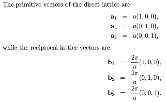
Fig 3. Primitive and reciprocal lattice vectors in sc.
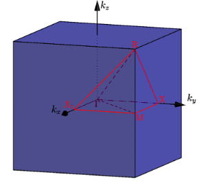
Fig 4. SC 1st Brilluoin zone.
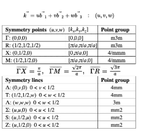
Fig 5. High symmetry points.
Plotting adiabatic magnon spectrum in the framework of Linear Spin Wave Theory
Use the UppASD graphical interface (ASDGUI) or the script enclosed in this course (plotsqw_course). Use option 2. File to print out “ams.HeisWire.out”.
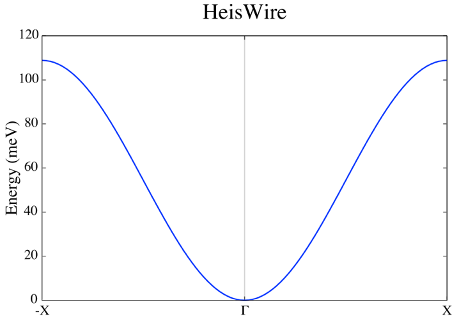
Fig 6. Adiabatic magnon spectra.
Plotting S(q,w)
Use the UppASD graphical interface (ASDGUI) or the script enclosed in this course (plotsqw_course). Use option 1 for S(q,w) or option 3 for S(q,w) with AMS. File to print out “sqw.HeisWire.out”.
do_sc Q           Measure spin correlation
sc_window_fun  2  Choice of FFT window function (1=box, 2=Hann, 3=Hamming, 4=Blackman-Harris)
sc_nstep 5000     Number of steps to sample
sc_step 8        Number of time steps between each sampling
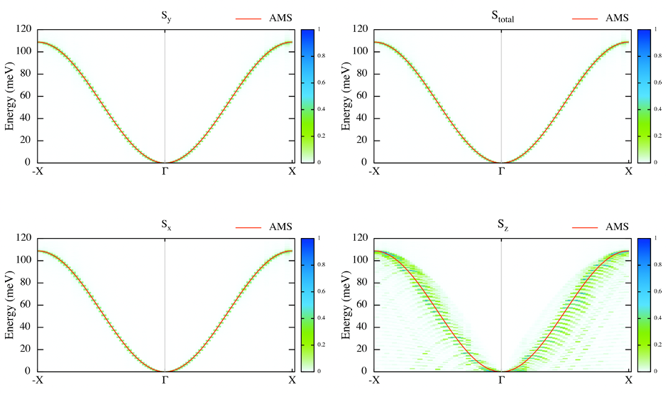
Fig 7. Structure factor together with AMS.
Questions and exercises:
Does it follows the analytical expression predicted by Linear Spin Wave Theory?
Tutorial 3: AFM Heisenberg nearest-neighbour spin chain
Collinear adiabatic magnon spectra and S(q,w)
The following tutorial shows every step necessary to calculate the spin wave spectrum and S(q,w) through the simple example of the antiferromagnetic spin chain. Notice that AMS in this case does not work for the primitive unit cell and it is necessary a magnetic supercell 2x1x1 of the crystal cell and define both spin directions in the supercell. Files are found in HeisChainAF folder.
Crystal & magnetic structure
Using the lines below with the indicated files, the crystal and magnetic structure are readily available, so that an 1D AFM Heisenberg chain is created. Have a look to posfile and momfile.
simid     HeisWire
ncell     1         1         100               System size
BC        0         0         P                 Boundary conditions (0=vacuum,P=periodic)
cell      1.00000   0.00000   0.00000
           0.00000   1.00000   0.00000
          0.00000   0.00000   2.000000
Sym       1                                     Symmetry of lattice (0 for no, 1 for cubic, 2 for 2d cubic, 3 for hexagonal)

posfile   ./posfile
exchange  ./jfile
momfile   ./momfile
do_prnstruct 1                                 Print lattice structure (0=no, 1=yes)
maptype   2                                    1=cartessian coordinates, 2=Direct coordinates
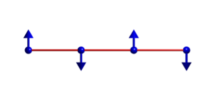
Fig 1. Crystal and magnetic texture.
Spin dynamics
Using the lines below, the systems is driven to the ground state by spin dynamics.
ip_mode   S                                     Initial phase parameters
ip_nphase 1
20000 1.0e-3 1e-16 4.0

mode      S                                     S=SD, M=MC
temp      1.0e-3                                Measurement phase parameters
damping   0.0010                                --
Nstep     45000                                 --
timestep  1.000e-15                             --

Fig 2. Energy versus number of iterations.
Spin wave spectrum
We calculate the spin wave spectrum (in this case, a collinear adiabatic magnon spectra) at the list of Q points (qfile). Use qmaker script.
do_ams Y                      Collinear Adiabatic magnon spectra
do_magdos N                   Generate magnon density of states

qpoints D                     Flag q-point generation(F=file,A=automa.,C=full cell,D=external
                              file with direct coordinates)
qfile   ./qfile               Path along the high symmetry points in the reciprocal space
The first Brilluoin zone of a simple cubic lattice
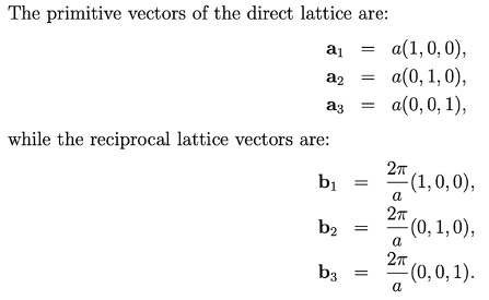
Fig 3. Primitive and reciprocal lattice vectors in sc.

Fig 4. SC 1st Brilluoin zone.

Fig 5. High symmetry points.
Plotting adiabatic magnon spectrum in the framework of Linear Spin Wave Theory
Use the UppASD graphical interface (ASDGUI) or the script enclosed in this course (plotsqw_course). Use option 2. File to print out “ams.HeisWire.out”.
Use only the primitive cell.
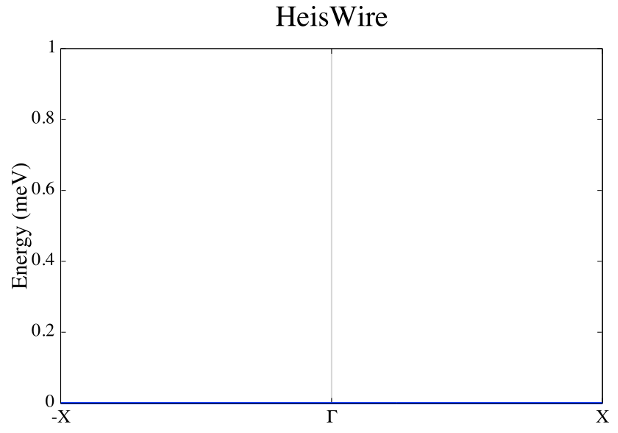
Fig 6. Adiabatic magnon spectra.
Use the magnetic supercell 2x1x1 of the crystal cell
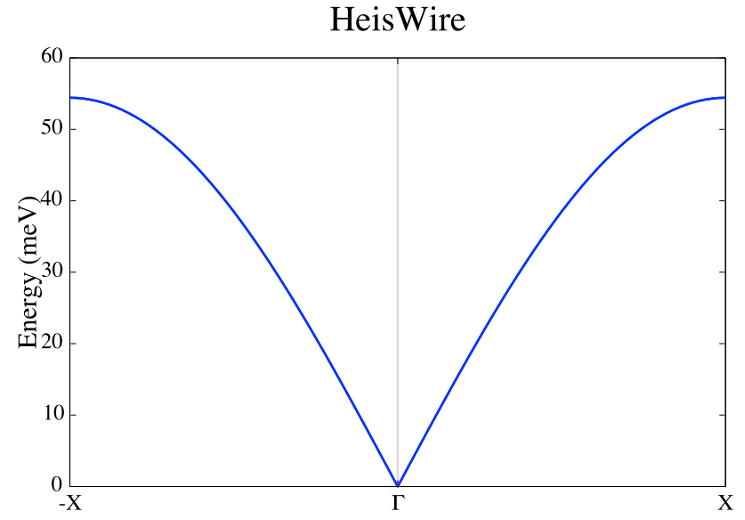
Fig 7. Adiabatic magnon spectra.
Plotting S(q,w)
Use the UppASD graphical interface (ASDGUI) or the script enclosed in this course (plotsqw_course). Use option 1 for S(q,w) or option 3 for S(q,w) with AMS. File to print out “sqw.HeisWire.out”.
do_sc Q           Measure spin correlation
sc_window_fun  2  Choice of FFT window function (1=box, 2=Hann, 3=Hamming, 4=Blackman-Harris)
sc_nstep 3000     Number of steps to sample
sc_step  15       Number of time steps between each sampling
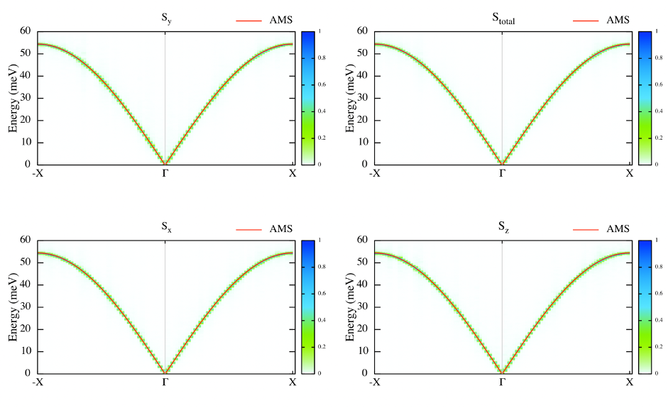
Fig 8. Structure factor with AMS.
Questions and exercises:
Does it follows the analytical expression predicted by Linear Spin Wave Theory? Why is linear around the center zone?
Calculate analytically the Energy/spin and show it is the same as the numerical result.
Tutorial 4: FM Heisenberg nearest-neighbour spin chain with DM interactions
Non-Collinear adiabatic magnon spectra and S(q,w)
The following tutorial serves as introduction to non-collinear AMS and shows every step necessary to calculate non-collinear spin wave spectrum and S(q,w) through the simple example of the ferromagnetic spin chain with DM interaction. Notice that AMS in this case does not work because the magnetic ground-state texture is non-collinear. Files are found in HeisChainDM folder.
Crystal & magnetic structure
Using the lines below with the indicated files, the crystal and magnetic structure are readily available, so that an 1D helical Heisenberg spin spiral is created. Have a look to posfile and momfile. Notice the system could be set up with just 1 atom per unit cell but, in this example, we use 4 atoms per unit cell just to help you to understand how to set up the dmfile for systems which have more than one atom per unit cell.
simid     HeisWire
ncell     1         1         100               System size
BC        0         0         P                 Boundary conditions (0=vacuum,P=periodic)
cell      1.00000   0.00000   0.00000
          0.00000   1.00000   0.00000
          0.00000   0.00000   4.00000
Sym       0                                     Symmetry of lattice (0 for no, 1 for cubic, 2 for 2d cubic, 3 for hexagonal)

posfile   ./posfile
exchange  ./jfile
momfile   ./momfile
dm        ./dmfile
do_prnstruct 1                                  Print lattice structure (0=no, 1=yes)
maptype 2
Mensemble 1                                     Number of samples in ensemble averaging
Initmag   3                                     (1=random, 2=cone, 3=spec., 4=file)
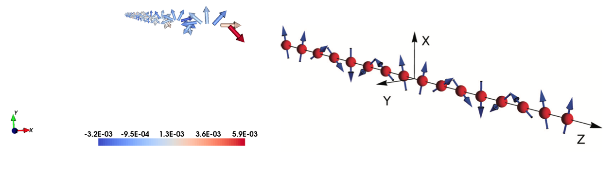
Fig 1. Crystal and magnetic texture.
Spin dynamics
Using the lines below, the systems is driven to the ground state by MonteCarlo.
ip_mode   M
ip_mcanneal 1
100000 1.0e-3

mode      S                                     S=SD, M=MC
temp      1.0e-3                                Measurement phase parameters
damping   0.0010                                --
Nstep     128000                                 --
timestep  1.000e-15                             --
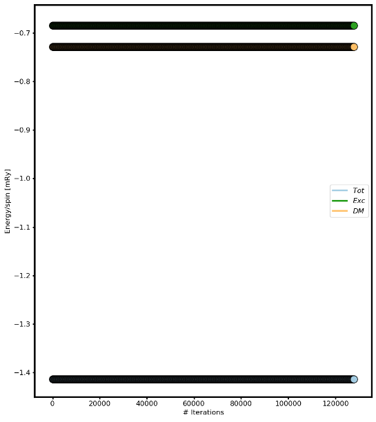
Fig 2. Energy versus number of iterations.
Spin wave spectrum
We calculate the non-collinear and collinear spin wave spectrum at the list of Q points (qfile) for comparison. Use qmaker script.
do_ams Y                      Collinear Adiabatic magnon spectra
do_diamag Y                   Non-Collinear Adiabatic magnon spectra

qpoints D                     Flag q-point generation(F=file,A=automa.,C=full cell,D=external
                              file with direct coordinates)
qfile   ./qfile               Path along the high symmetry points in the reciprocal space
The first Brilluoin zone of a simple cubic lattice

Fig 3. Primitive and reciprocal lattice vectors in sc.
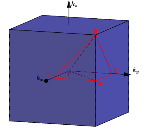
Fig 4. SC 1st Brilluoin zone.
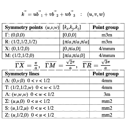
Fig 5. High symmetry points.
Plotting adiabatic magnon spectrum in the framework of Linear Spin Wave Theory
Use the UppASD graphical interface (ASDGUI) or the script enclosed in this course (plotsqw_course). Use option 2. File to print out “ams.HeisWire.out”.
Collinear AMS
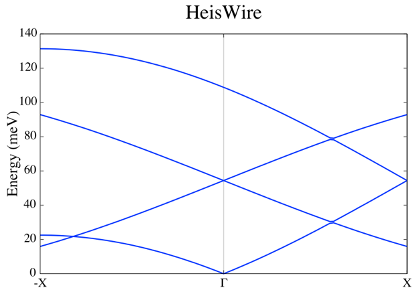
Fig 6. Collinear Adiabatic magnon spectra.
Non-Collinear AMS
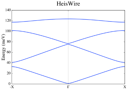
Fig 7. Non-collinear Adiabatic magnon spectra.
Plotting S(q,w)
Use the UppASD graphical interface (ASDGUI) or the script enclosed in this course (plotsqw_course). Use option 1 for S(q,w), option 4 for S(q,w) with NC_AMS and option 5 S(q,w) with AMS. File to print out “sqw.HeisWire.out”.
do_sc Q                                         Measure spin correlation
sc_nstep 8000                                   Number of steps to sample
sc_step  16                                     Number of time steps between each sampling
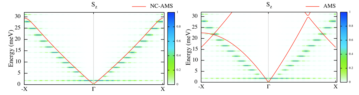
Fig 8. Structure factor together with non-Collinear AMS and collinear AMS.
Questions and exercises:
Do you understand why Collinear AMS failed in this case?
Tutorial 5: Kagome system with DM interactions
Non-Collinear adiabatic magnon spectra and S(q,w)
The following tutorial serves as introduction to non-collinear AMS when the unit cell is commensurate with the magnetic unit lattice. It shows every step necessary to calculate non-collinear spin wave spectrum and S(q,w). Files are found in Kagome_ncAMS folder.
Crystal & magnetic structure
Using the lines below with the indicated files, the crystal and magnetic structure are readily available, so that an Kagome system with DM interaction is created. Have a look to posfile and momfile, etc.
simid  kagome_T
ncell    66 66 1
BC         P P 0
cell     1.000000000000    0.000000000000    0.000000000000
        -0.500000000000    0.866025403784    0.000000000000
         0.000000000000    0.000000000000    10.00000000000

Sym        0

posfile    ./posfile
posfiletype D               C=Cartesian or D=direct coordinates in posfile
momfile    ./momfile
exchange   ./jfile

maptype 2
do_jtensor 1
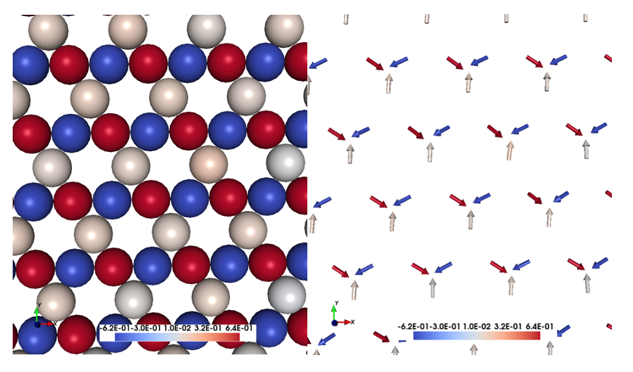
Fig 1. Crystal and magnetic texture.
Spin dynamics
Using the lines below, and using a momfile with previous minimization, the system is already in the ground-state. This is just to speed up the simulation time.
ip_mode N
ip_mcanneal 2
10000 100.0001
10000 0.0001

mode      S                                     S=SD, M=MC
temp      0.0001
Nstep     60000
damping   0.001
timestep  1d-16
Spin wave spectrum
We calculate the non-collinear spin wave spectrum (in this case, a collinear adiabatic magnon spectra) at the list of Q points (qfile). Use qmaker script.
do_ams Y                      Collinear Adiabatic magnon spectra
do_diamag Y                   Non-Collinear Adiabatic magnon spectra

qpoints D                     Flag q-point generation(F=file,A=automa.,C=full cell,D=external
                              file with direct coordinates)
qfile   ./qfile               Path along the high symmetry points in the reciprocal space
The first Brilluoin zone of a hexagonal lattice
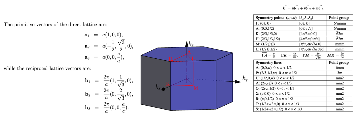
Fig 2. Primitive and reciprocal lattice vectors in hcp with 1st Brilluoin zone and High symmetry points.
Plotting adiabatic magnon spectrum in the framework of Linear Spin Wave Theory
Use the UppASD graphical interface (ASDGUI) or the script enclosed in this course (plotsqw_course). Use option 4. File to print out “ncams.kagome_T.out”.
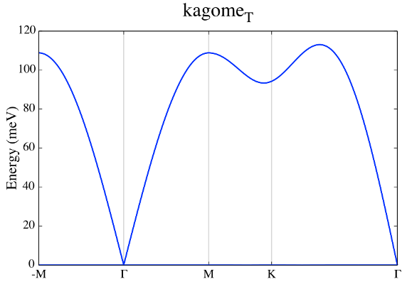
Fig 3. Non-Collinear AMS.
Plotting S(q,w)
Use the UppASD graphical interface (ASDGUI) or the script enclosed in this course (plotsqw_course). Use option 1 for S(q,w), option 4 for S(q,w) with NC_AMS. File to print out “ncams.kagome_T.out” and “sqw.kagome_T.out”.
do_sc  Q
sc_nstep 500
sc_step   90
do_sc_local_axis B             Perform SQW along local quantization axis (SA) (Y/N/B)
                               B--> B_effxSA
sc_window_fun 2                Choice of FFT window function (1=box, 2=Hann, 3=Hamming,
                               4=Blackman-Harris)
sc_average N                   Averaging of S(q,w): (F)ull, (E)ven, or (N)one
do_sc_tens N                   Print the tensorial values s(q,w) (Y/N)

qpoints D
qfile ./qfile
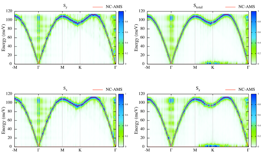
Fig 4. Structure factor together with non-Collinear AMS.
Questions and exercises:
Is there only one branch?
Seems linear around Gamma point but J is FM? Why is that? Shouldn´t be parabolic?
Tutorial 6: Triangular system with AFM interactions
Non-Collinear adiabatic magnon spectra and S(q,w)
The following tutorial serves as how to use non-collinear AMS for systems that are not commensurate with the magnetic unit cell. It shows every step necessary to calculate non-collinear spin wave spectrum and S(q,w). Files are found in Triangular_ncAMS folder.
Crystal & magnetic structure
Using the lines below with the indicated files, the crystal and magnetic structure are readily available, so that an AFM triangular lattice is created. Have a look to posfile and momfile, etc.
simid  triang_T
ncell    66 66 1
BC         P P 0
cell     1.000000000000    0.000000000000    0.000000000000
        -0.500000000000    0.866025403784    0.000000000000
         0.000000000000    0.000000000000    10.00000000000

Sym        3                Symmetry of lattice (0 for no, 1 for cubic, 2 for 2d cubic, 3 for hexagonal)

posfile    ./posfile
posfiletype D                C=Cartesian or D=direct coordinates
momfile    ./momfile
exchange   ./jfile

maptype 2
do_jtensor 1
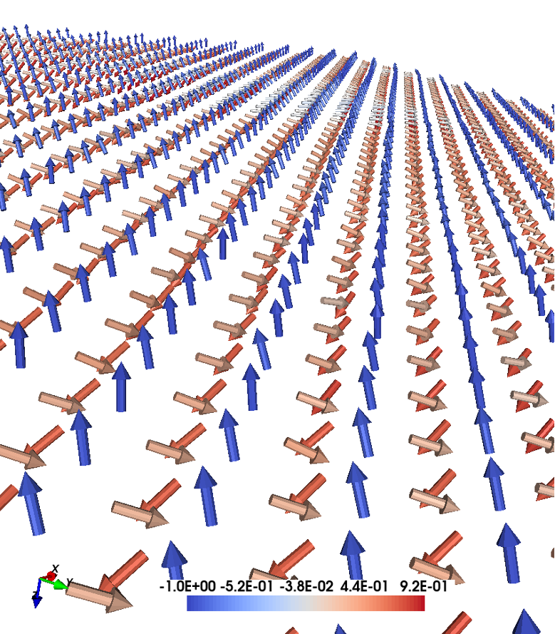
Fig 1. Crystal and magnetic texture.
Spin dynamics
Using the lines below the system is evolved in time. Notice that in the initial phase, we use a minimization of the spin-spiral energy, and by doing that, the ordering wave vector is calculated. In a second calculation, the adiabatic magnon spectra is calculated by using the already calculated ordering wave vector of the spin spiral based on the direction provided by the spin vector qm_svec and qm_nvec which is perpendicular to the given spin direction.
ip_mode Q                                Activate qminimizer
                                         minimize spin-spiral energy
                                         calculate ordering wave vector, etc.
ip_nphase 1
50000 0.00000 1.0e-16 5.0
10000 300.0001 1.0e-16 5.0
10000 100.0001 1.0e-16 5.0
10000 10.0001  1.0e-16 5.0
20000 1.0001   1.0e-16 5.0
50000 0.00000 1.0e-16 5.0

mode      S                                     S=SD, M=MC
temp      0.1
Nstep     59500
damping   0.001
timestep  1e-16
qm_nvec 0 0 1                             Unit-vector perpendicular to spins
qm_svec 0 1 0                             Direction of the spin
Spin wave spectrum
We calculate the non-collinear spin wave spectrum (in this case, a collinear adiabatic magnon spectra) at the list of Q points (qfile). Use qmaker script.
do_diamag Y                   Non-Collinear Adiabatic magnon spectra

qpoints D                     Flag q-point generation(F=file,A=automa.,C=full cell,D=external
                              file with direct coordinates)
qfile   ./qfile               Path along the high symmetry points in the reciprocal space

nc_qvect 0.330000 0.571577 0.000000   Ordering wave vector
nc_nvect 0.0 0.0 1.0                  Pitch-vector along z and the moments rotate
                                      in the xy-plane
qm_nvec 0 0 1                             Unit-vector perpendicular to spins
qm_svec 0 1 0                             Direction of the spin
The first Brilluoin zone of a hexagonal lattice

Fig 2. Primitive and reciprocal lattice vectors in hcp with 1st Brilluoin zone and High symmetry points.
Plotting adiabatic magnon spectrum in the framework of Linear Spin Wave Theory
Use the UppASD graphical interface (ASDGUI) or the script enclosed in this course (plotsqw_course). Use option 7. File to print out “ncams.kagome_T.out”, “ncams+q.triang_T.out” and “ncams-q.triang_T.out”
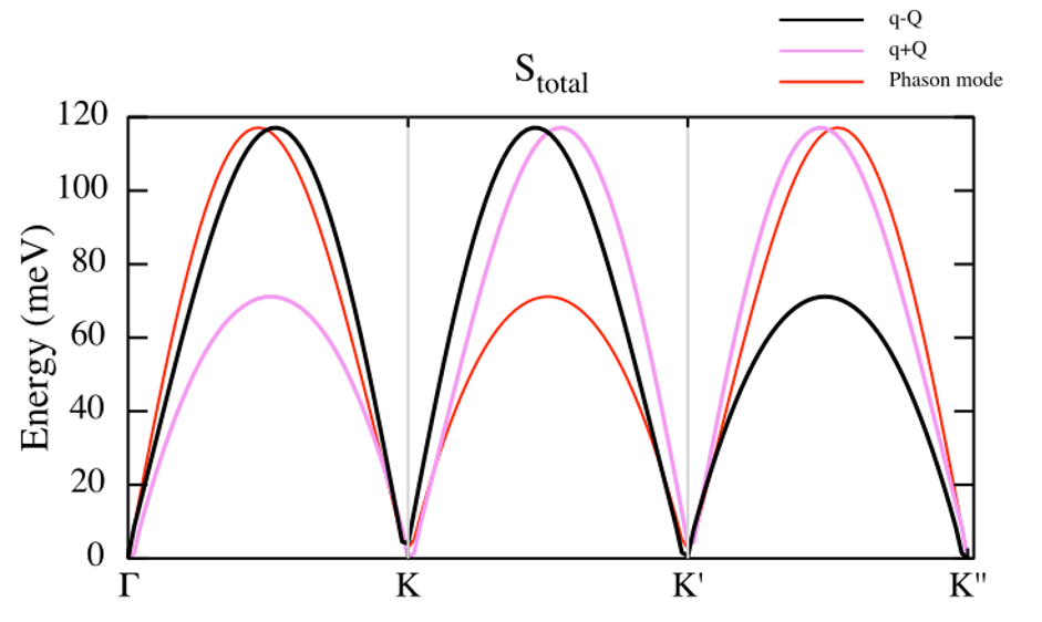
Fig 3. Non-Collinear AMS.
Plotting S(q,w)
Use the UppASD graphical interface (ASDGUI) or the script enclosed in this course (plotsqw_course). Use option 1 for S(q,w), option 6 for S(q,w) with NC_AMS+Q. File to print out “ncams.kagome_T.out”, “sqw.kagome_T.out”,” ncams+q.triang_T.out” and “ncams-q.triang_T.out”.
do_sc  Q
sc_nstep 700
sc_step   85
do_sc_local_axis B             Perform SQW along local quantization axis (SA) (Y/N/B)
                               B--> B_effxSA
sc_window_fun 2                Choice of FFT window function (1=box, 2=Hann, 3=Hamming,
                               4=Blackman-Harris)
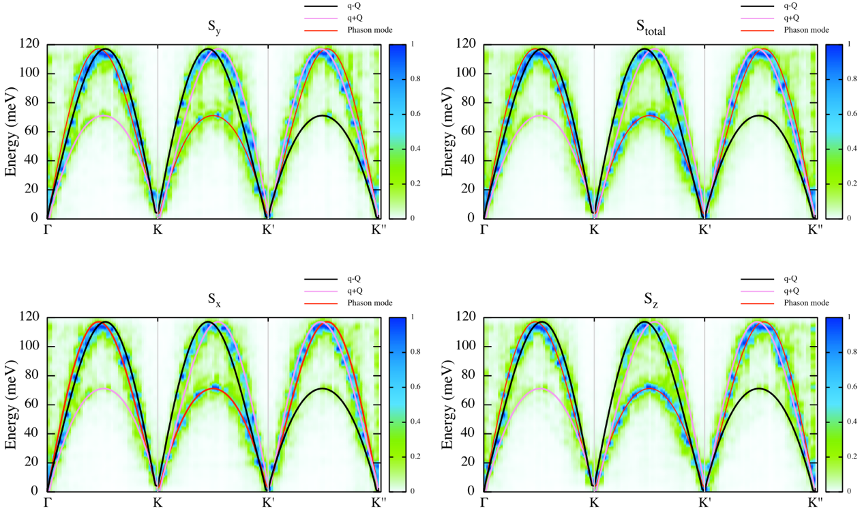
Fig 4. Structure factor together with non-Collinear AMS with non-zero ordering wave vector.
Questions and exercises:
Why we have 3 branches, with just 1 atom per unit cell?
Is it the profile of an antiferromagnet around the Gamma point?
Some preliminary and useful equations:
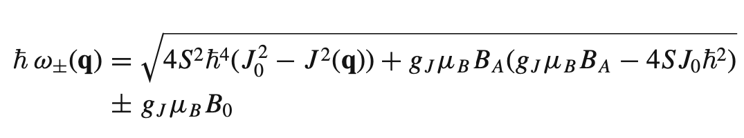
Eq 1. Excitation energy for spin waves in an anisotropic antiferromagnet.
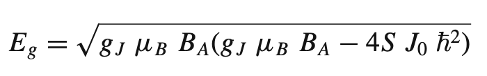
Eq 2. Energy gap due to the anisotropy.
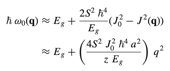
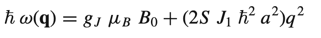
Eq 3. Excitation energy for spin waves in an anisotropic ferromagnet.
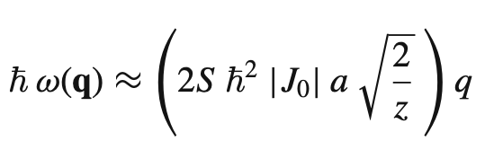
Eq 4. Excitation energy for spin waves in an isotropic antiferromagnet.
Eq 5. Excitation energy for spin waves in an isotropic ferromagnet.