Finite temperatures
Statistics
In this exercise we will investigate how statistics affect simulated measurables.
A single spin with an uniaxial anisotropy has a bi-stable, Ising like, magnetic state. At finite temperatures the stability of the magnetic state is not finite but follows an exponential (Arrhenius) relaxation behaviour. As seen in the lecture, ensemble averaging can be crucial for the analysis of such systems.
Investigate the amount of statistics that is needed to say something relevant about the life time of the magnetic state of the system.
Does the need of statistics change with system parameters? (temperature, anisotropy, external field)
Extra: Can you fit the relaxation behaviour to an Arrhenius function?
You can do a similar analysis for a finite 1d-chain by either modifying the single spin example, or starting from the SimpleSystems/HeisChain example.
Is there a difference by performing ensemble averaging compared to just increasing the system size?
Does the exchange interaction magnitude affect the stability of the spin chains?
An accessible article for those interested in spin chains and statistics can be found here: A. Vindigni Inorganica Chimica Acta, 361 3731 (2008).
Thermalization
In this exercise the thermalization rates in spin simulations will be investigated.
As mentioned in the lecture, thermalising the system before performing measurements is crucial for ensuring relevant results. Here we will investigate this for a simple cubic model system.
The initial inpsd.dat file looks as follows
simid simpcube
ncell     10        10       10                 System size
BC        P         P         P                 Boundary conditions (0=vacuum, P=periodic)
cell      1.00000   0.00000   0.00000
          0.00000   1.00000   0.00000
          0.00000   0.00000   1.00000
Sym       1                                     Symmetry of lattice (0 for no, 1 for cubic, 2 for 2d cubic, 3 for hexagonal)
do_prnstruct 1

posfile      ./posfile
momfile      ./momfile
exchange     ./jfile

Initmag     3                                   Initial config of moments (1=random, 2=cone, 3=spec., 4=file)

ip_mode     S
ip_mcanneal 1
            5000  300.0 1.00e-16 0.95

mode        S
Temp        300.00          K                    Temperature of the system
hfield      0.00000   0.00000   0.00000          Static H field

damping     0.01                                 Damping parameter (gamma)
nstep       10000                                Number of time-steps
timestep    1.000e-16       s                    The time step-size for the SDE-solver

plotenergy  1                                    Sample energies
do_avrg     Y                                    Measure averages
do_cumu     Y                                    Sample cumulative averages
do_spintemp Y                                    Measure spin temperature
and the almost trivial posfile and momfile are written as
1 1 0.000000 0.000000 0.000000
1 1 1.00 0.0 0.0 1.0
The jfile, that will be changed during the exercise initially can look like
1 1  1.0       0.0       0.0       0.80000000000000
1 1  1.0       1.0       0.0       0.50000000000000
i.e. including nearest and next-nearest neighbours on the cubic lattice. Notice that since sym 1 is given in inpsd.dat, the jfile can be kept to a minimum of two lines.
Starting with the inputs as defined above, vary the simulation method and damping (where applicable) to investigate the thermalization rate of the system.
Is the thermalization faster when going from low to high temperatures or vice versa? Anything particular happening around Tc?
Change the sign of the next-nearest neighbour and redo the study. Is the magnetization a good measurable for determining the thermalization now?
Phase diagrams
Obtaining the M vs T relationship is probably the most common use case for Monte Carlo simulations on spin systems. In this exercise you can compare the MC functionalities of UppASD with a the ALPS package.
The system in question is here the 2d square lattice with NN exchange couplings.
To compare with other model implementations this example uses the aunits Y flag which sets the temperature unit to the exchange strength J instead of Kelvin.
The inpsd.dat will here look as follows (to start with). Note the TEMP entries for initial and measurement temperatures.
simid  scHeis64
ncell     64 64 1
BC        P         P         0                 Boundary conditions (0=vacuum,P=periodic)
cell      1.00000   0.00000   0.00000
          0.00000   1.00000   0.00000
          0.00000   0.00000   1.00000
Sym       1                                     Symmetry of lattice (0 for no, 1 for cubic, 2 for 2d cubic, 3 for hexagonal)

aunits Y
posfile    ./posfile
exchange   ./jfile
momfile    ./momfile
do_prnstruct 1

Mensemble 1
Initmag   3                                     (1=random, 2=cone, 3=spec., 4=file)

ip_mode   M                                     Initial phase parameters
ip_temp   TEMP                                  --
ip_mcNstep     5000                            --

mode      M                                     S=SD, M=MC
temp      TEMP                                  Measurement phase parameters
mcNstep   5000                                --

do_avrg   Y                                     Measure averages
plotenergy 1
do_cumu Y
and the posfile and momfile, and jfile files looks as
1 1 0.0 0.0 0.0
1 1 1.00000 0.0 0.0 1.0
1 1 1.0 0.0 0.0 0.5000
Again, note that with aunits Y the exchange interaction in jfile is not defined in mRy but in the dimensionless energy scale of J (which is not Joule either).
In order to obtain the full M(T) curve, several simulations are needed at consecutive temperatures.
This is preferably scripted, like in this example where we use a simple bash script runme.sh
#!/bin/bash

for Temp in 0.1 0.2 0.3 0.4 0.5 0.6 0.7 0.8 0.9 1.0 1.1 1.2 1.3 1.4 1.5 1.6 1.7 1.8 1.9 2.0
do
    mkdir T$Temp/
    echo "Temp: " $Temp
    cp Base/* T$Temp/
    cd T$Temp/
    gsed -i "s/TEMP/$Temp/g" inpsd.dat
    ${SD_BINARY} > out.log
    cd ..
done
Here you either need to replace the ${SD_BINARY} expression, or export the location of your UppASD binary as the environment variable with the same name.
You also need to use the same directory structure as intended, i.e. put the input files in a directory called Base and the runme.sh
script in the directory below.
Run the script and plot the resulting M(T) curve.
Compare with the reference data in the
sc_64_ALPS.datfileAre the simulation parameters “good enough” or are more thermalization/sampling steps needed to obtain an accurate M(T) curve?
Minimization
Ground state determination is another situation where Monte Carlo and Atomistic spin dynamics simulations are used extensively. For isotropic ferromagnets this is usually a trivial task but for systems with exchange frustration and/or strongly anisotropic systems the ground state search can prove quite demanding.
In this exercise you will examine different kinds of magnetic systems with the task of finding their respective ground states.
Anisotropic systems
The first example starts from the square lattice of the previous exercise, but this time we will add a uniaxial anisotropy to the system.
Copy the input files from the previous exercise and add a uniaxial anisotropy with a strength of 0.4J , where J still is the
dimensionles unit of energy as earlier. An anisotropy is added by including the keyword anisotropy ./kfile to inpsd.dat and
creating the anisotropy file kfile as per below. Also start with the jfile that only had positive exchange couplings.
1 1 -0.40 0.00 0.00000 0.00000 1.00000 0.0
Note that you can give all input files besides inpsd.dat more descriptive names if wanted.
With the anisotropy included, simulate the system starting from the ferromagnetic configuration by using
initmag 3and relax the system to a temperature approaching zero. You can visualize the structure using the GUI, or if it fails to run with theASD_Tools/myRestart3.pyscript provided in the Github repository.< myRestart3.py
This should give you a ferromagnetic order of the full sample, as expected.
Now change the starting guess to a fully disordered state by using
initmag 1and redo the relaxation. What state do you end up with?
The anisotropies in the system causes large energy barriers that can not be overcome at low temperatures. So unless the starting guess is good there is a risk that one ends up in a local minimum instead of the global one. To overcome these barriers one can employ higher temperatures which is typically done with the “Simulated annealing” (SA) approach, where one performs consecutive initial phase runs, starting from a high temperature and gradually reducing the temperature to the target value.
In UppASD, this is preferably done using the ip_mcanneal or ip_nphase constructs. An example is seen below.
ip_mode H
ip_mcanneal 5
1000 2.0
1000 0.5
1000 0.1
1000 0.01
1000 0.001
There are no global recipies for the optimal number if anneal sweeps and the temperature distibution so here empirical experience is your friend.
Try different SA sequences and see if you can relax the anisotropic system to its ferromagnetic ground state.
Dzyalosinskii-Moriya systems
Also without anisotropy, ground state relaxation can prove a formidable task.
simid SCsurf_T
ncell     128 128 1
BC        P         P         0                 Boundary conditions (0=vacuum,P=periodic)
cell      1.00000   0.00000   0.00000
          0.00000   1.00000   0.00000
          0.00000   0.00000   1.00000

do_prnstruct 2
posfile   ./posfile
exchange  ./jfile
momfie    ./momfile
dm        ./dmfile


Initmag   1                                     (1=random, 2=cone, 3=spec., 4=file)

ip_mode N
ip_mcanneal 0

mode      S                                     M for MC and S for SD
temp      0.000
damping   0.500
Nstep     5000
timestep  1.000e-15       s                    The time step-size for the SDE-solver


plotenergy   1
do_avrg      Y
do_cumu      Y
and the posfile, jfile, momfile as below
1 1 0.0 0.0 0.0
1 1  1.0       0.0       0.0      1.00000
1 1 -1.0       0.0       0.0      1.00000
1 1  0.0       1.0       0.0      1.00000
1 1  0.0      -1.0       0.0      1.00000
1 1 1.0 0.1 0.0 1.0
Now we also have a Dzyaloshinskii-Moriya (DM) file dmfile that looks like
1 1  1.0000  0.0000 0.0000  0.81650  0.00000  0.00000
1 1 -1.0000  0.0000 0.0000 -0.81650 -0.00000 -0.00000
1 1  0.0000  1.0000 0.0000  0.00000  0.81650  0.00000
1 1  0.0000 -1.0000 0.0000 -0.00000 -0.81650 -0.00000
where the first five columns are the same as for a regular jfile i.e. atom sites and distance vector \(\mathbf{R}_{ij}\).
The remaining three columns define the DM interaction vector \(\mathbf{D}_{ij}\). This system with ferromagnetic exchange and significant
DM interactions has a spin-spiral ground state as shown below.
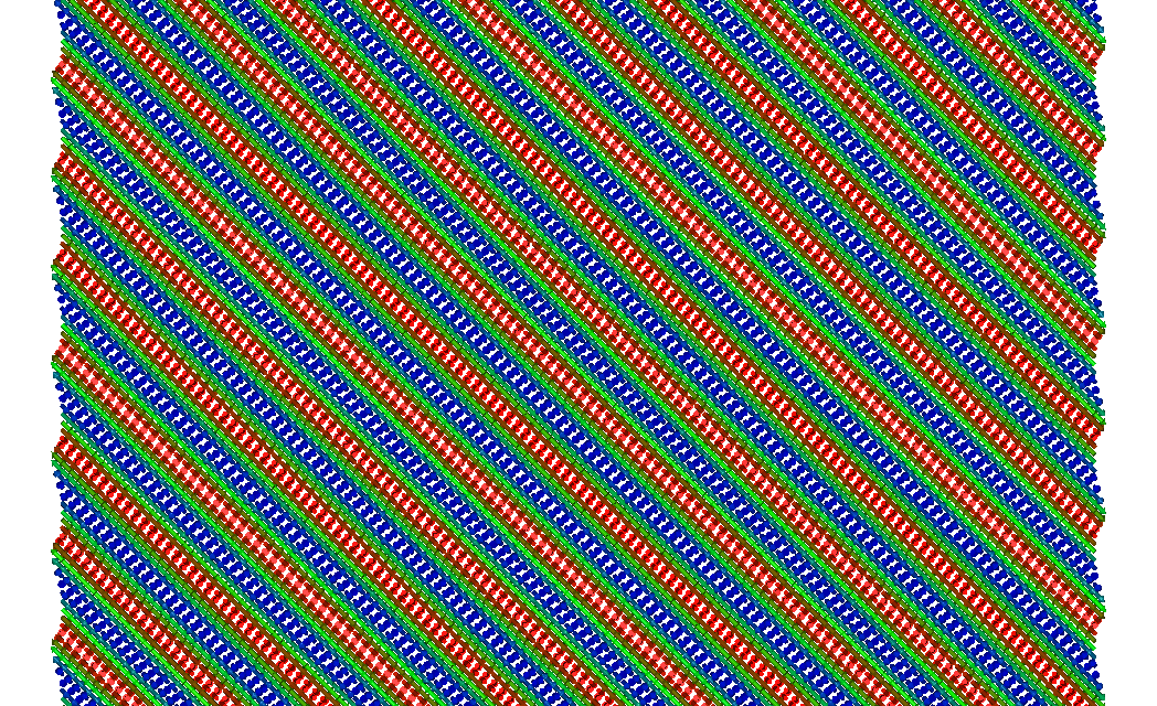
Fig. 1 Spin spiral ground state for a DM system.
For this setup, start from a random configuration with
initmag 1and relax the structure. What end state do you get?If you do not get the spiral state, try to obtain it with simulated annealing. How close can you come? Is the energy stabilizing?
Glassy systems
As a final challenge, lets consider a spin glass system. A simple yet illustrative model for a spin glass system is given by the Edwards-Anderson model, where a nearest neighbour Hamiltonian on a cubic lattice, but with random exchange interactions are used.
The UppASD code can model Edwards-Anderson spin glasses by the keywords ea_model T and ea_sigma XX where ea_sigma contols
the width of the Gaussian distribution of the randomized exchange interactions. Disregarding the ea_sigma keyword for now,
we can define a simple cubic system with randomized exchange with the following inpsd.dat
simid bccFe100
ncell     10        10       10                 System size
BC        P         P         P                 Boundary conditions (0=vacuum, P=periodic)
cell      1.00000   0.00000   0.00000
          0.00000   1.00000   0.00000
          0.00000   0.00000   1.00000
Sym       0
do_prnstruct 2

posfile    ./posfile
momfile    ./momfile
exchange   ./jfile

Initmag   1                                     Initial config of moments (1=random, 2=cone, 3=spec., 4=file)

ip_mode   N
ip_mcanneal 1
          10000 100.0 1.00e-16 0.95
          100 100.0 1.00e-16 0.95
          100 100.0 1.00e-16 0.95

mode      M
Temp      0.001         K                     Temperature of the system
hfield    0.00000   0.00000   0.00000           Static H field
mcnstep   10000                                Number of time-steps

do_avrg   Y                                     Measure averages
plotenergy 1
do_cumu Y

ea_model T

do_autocorr Y
acfile ./acfile
While the posfile and momfile are made as easy as possible
1 1 0.000000 0.000000 0.000000
1 1 1.00 1.0 0.0 0.0
Even though the exchange interactions will be randomized, we still have to set up a Hamiltonian with existing couplings since only
the magnitude and not the directions will be randomized. Thus we use the following jfile
1 1  1.0       0.0       0.0       1.00
1 1 -1.0       0.0       0.0       1.00
1 1  0.0       1.0       0.0       1.00
1 1  0.0      -1.0       0.0       1.00
1 1  0.0       0.0       1.0       1.00
1 1  0.0       0.0      -1.0       1.00
With the glassy system setup. we end this exercise session with a friendly competition:
Without changing the system size and Hamiltonian, apply your thermalization and minimization skills to get the lowest possible energy for this system.
The participant with the lowest energy will get a symbolic price during the conference dinner.